techBASIC as a Graphing Calculator

techBASIC: The Power-User’s Graphing Calculator
Graphing calculators have been a staple of math and science classes for decades, and for good reason. It’s easier to grasp basic concepts and to understand what is happening with a function if you can see it, and that’s what a graphics calculator is all about. techBASIC is the ultimate power-user’s graphics calculator. It’s almost as easy to use as a traditional physical graphing calculator, but offers far more options, better resolution, and better control over the function itself.
This blog takes a look at how to use techBASIC as a graphing calculator. You’ll discover that almost no programming is needed to get the same functionality you get form a graphing calculator, and with command of the simple IF statement, you can do far more with techBASIC than you can do with graphing calculators without programming.
Getting Started with Graphing in techBASIC


where

It’s a function used to demonstrate how to manipulate 3D data in techBASIC. Here’s a review of the touch-based options you can use to manipulate the graph.
Wednesday, May 16, 2012

Graphing different functions in 2D and 3D is pretty easy. All you do is calculate the value and assign it to f. There are really only two differences between the way you would write the equation in mathematics and the way it is written in techBASIC. The first is that multiplication is not implied. For example, it’s common to write something like

and expect that it is understood that 5 is multiplied by x. In BASIC, you have to put the multiplication in explicitly, like this:
f = 1.3 + 5*x
The other difference is that BASIC only uses the characters on a standard keyboard, so it doesn’t use symbols like √ for square root. As you’ve seen, BASIC uses a function, instead, so

becomes
d = SQR(x*x + y*y)
in BASIC. Here’s a quick reference list of the functions that are most commonly used in functions.

ABS
ATAN ATAN
COS
EXP
INT
LOG
SGN SGN
SIN
SQR
TAN

FUNCTION f(d)
f = TAN(d)
END FUNCTION

FUNCTION f(d)
f = SQR(d)
END FUNCTION
As you can see, if the function has no value, techBASIC doesn’t draw it. Of course, with a simple change, you can test for this condition and plot something there, too, perhaps reflecting the positive value.
FUNCTION f(d)
IF d < 0 THEN
f = -SQR(-d)
ELSE
f = SQR(d)
END IF
END FUNCTION
Creating Your Own Programs
While there is little reason to create a program from scratch to graph functions, you might want to create several programs to plot several different functions. The easy way to do that is to start with an existing program and copy it.
If you have a physical keyboard, hold down the Command key and press A. This selects everything in the program. Now hold down the Command key and press C. This copies everything in the program.

If you don’t have a physical keyboard, tap somewhere on the screen, wait a moment, and tap the same place again. You’ll get the option to Select, Select All or Paste. (If you see different options, you tapped quickly enough that the taps were treated as a double-tap. Try again in a new location, but wait a bit longer between taps.) Tap Select All.


The new program is empty. Tap two times, and you will get a Paste button. Press that button, and you will have a copy of the original program. Change the function to whatever it should be for this program, and you have a new program for your specific function.
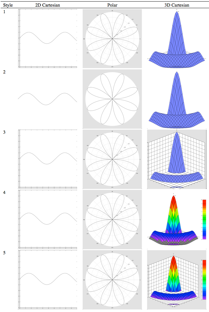
Graphing Options
There are an amazing number of options you can use for a graph. Let’s take a look at the ones used in the Sinx_x program to get an overview.
p.setTitle("f(x, y) = 10*sin(r)/r; r = sqrt(x*x + y*y)")
A few lines into the program, you see this line, which sets the title displayed across the top of the graph. You can delete this line entirely, and get more room for the graph itself, or change the text between the quote marks to change the title of the graph. This is one of the functions that applies to the entire graph. Here’s another one.
p.setGridColor(0.85, 0.85, 0.85)
This sets the grid color, which is the color of the lines that appear on the axis. Like all colors, this call breaks the color down into the red, green and blue components, with each varying between 0 (no color) to 1 (full intensity). The color shown is a light gray.
p.setsurfacestyle(3)

1Solid color
2No mesh is drawn
3Use false color
The rainbow effect you see on many 3D functions in techBASIC uses false color to help highlight the Z value of a function. The default is a solid color that can be changed with setSurfaceColor, or you can choose option 2, which doesn’t draw the surface at all—that let’s you see the lines that divide the normally colored surface, without seeing the surface itself.
Check out the documentation for setSurfaceColor for a moment by tapping Plot, then setSurfaceColor. There are four parameters, not just the normal three for red, green, and blue. The optional fourth parameter, called alpha, is the opacity of the color. If you leave it at the default value of 1, the color is opaque, so anything behind the surface is hidden. A really useful effect is to use a translucent color so you can see partially through the surface, seeing some of the features behind it. It’s like looking through a colored plastic sheet and seeing some of the detail behind it. Try changing
to
p.setsurfacestyle(1)
p.setSurfaceColor(0, 0, 1, 0.5)
to see this effect. Remember to change the function back to a 3D function, too!
The next line in the program is
p.setAxisStyle(5)
This selects among the various axis styles. Now that you know how to use the documentation, you can quickly see that the styles are
1Standard Cartesian or Polar axis
2No axis is drawn
3A box style axis
4A standard axis with color legend
5A box axis with color legend
This is where the PDF user’s manual is nice. While a little experimenting will help you figure out any options that are not obvious, the PDF manual has this table, which makes the options clear at a glance.
Absolute value
Single-argument arc tangent. The argument is y/x, and the result is in radians. The reference manual gives a handy function to calculate a two-argument arc tangent.
Cosine. The argument is in radians.
Returns the natural exponent of the argument, ex.
Returns the largest integer that is less than or equal to the argument.
Returns the natural logarithm of the argument.
Returns -1 if the argument is less than 0, 0 if the argument is 0, and 1 if the argument is greater than 0.
Sine. The argument is in radians.
Square root.
Tangent. The argument is in radians.
Of course, there are lots of other options. Now that you know how to use the help system, you can explore these if you like—or ignore them if you’d rather not deal with that level of programming detail.
Plotting Multiple Functions
What if you want to plot more than one function at the same time? That’s really not difficult. While it works in both 2 and 3 dimensions, let’s stick with 2 dimensions for a moment. Change the function that will be plotted to sin(x)/x, like this:
FUNCTION f(x)
IF x = 0 THEN
f = 1
ELSE
f = SIN(x)/x
END IF
END FUNCTION
Test it to make sure you get what you expect. Now let’s compare this to the sine. We’ll need a new function, so add this to the end of the program:
FUNCTION g(x)
g = SIN(x)
END FUNCTION
That adds the function, but we still need to add the plot of this function to the graph. Back up in the program, you’ll find the lines
! Add the function.
DIM func AS PlotFunction
func = p.newFunction(FUNCTION f)
Copy those and paste a copy below these three lines, then change them to look like this:
! Add the function.
DIM func AS PlotFunction
func = p.newFunction(FUNCTION f)

DIM funG AS PlotFunction
funG = p.newFunction(FUNCTION g)
This creates a new function and adds it to the plot. You might also want to add a little color so it is easier to tell the functions apart. Looking at the documentation, you’ll find the setColor call listed for the PlotFunction class. Let’s make sin(x)/x red, and sin(x) green, like this:
! Add the function.
DIM func AS PlotFunction
func = p.newFunction(FUNCTION f)
func.setColor(1, 0, 0)
! Add the function g.
DIM funG AS PlotFunction
funG = p.newFunction(FUNCTION g)
funG.setColor(0, 1, 0)
Other Coordinate Systems
So far we’ve worked in Cartesian coordinates, but techBASIC also handles polar coordinates in 2D, and spherical and cylindrical coordinates in 3D. Let’s start with polar coordinates, drawing a simple spiral. Polar functions take the angle as the parameter and return the radius, so the function looks like this:

g = x
END FUNCTION
That looks a lot like the functions we’ve worked with already, and it is. The difference is in how we create the plot. Instead of using the newFunction call, we’ll use newPolar. Everything else looks the same.
DIM func AS PlotFunction
func = p.newPolar(FUNCTION f)
If you started with the program from the last section that plots two functions, you’ll still see the plotted over the polar function, too! This shows that you can mix coordinate systems. That’s not usually what you want, so you might delete the second function, but it does work. You might also notice that the axis for polar functions is pretty different from the axis for Cartesian coordinates. If you add two functions to a plot, the default axis will be the axis for the first function added. You can change it with the setAxisKind call. Adding this new line changes back to a standard Cartesian axis.
DIM func AS PlotFunction
func = p.newPolar(FUNCTION f)
p.setAxisKind(1)
Be sure to set the axis kind after adding the first function, or techBASIC will change the axis kind again when you add the function.
With the model you’ve just seen for polar coordinates, you can probably anticipate how you will use cylindrical and spherical coordinates. Change the lines that create the function from

func = p.newPolar(FUNCTION f)
p.setAxisKind(1)
to
DIM func AS PlotFunction
func = p.newCylindrical (FUNCTION f)
and change the function to this one, which plots a cone.
FUNCTION f(r, theta)
f = r
END FUNCTION
For spherical coordinates, change newCylindrical to newSpherical:

func = p.newSpherical (FUNCTION f)
and change the function to something that makes sense in spherical coordinates. Here’s a fun function that plots the first rotation of a sea shell!
FUNCTION f(theta, phi)
f = phi
END FUNCTION
Where to Go From Here
You’ve learned a lot about manipulating graphs in techBASIC. Along the way, you’ve even learned a lot about programming. That’s the beauty of techBASIC. You can learn just a little programming to do a specific task, but as the tasks change, you’ll put those small lessons together, increasing your ability to program as you go. Since you are learning BASIC, you’re also learning a language you can use in many other settings, like writing Excel spreadsheet macros.
There are lots of options and functions we did not explore here, but you also learned to use the help system to find other options. Perhaps you did not download the PDF reference manual. If not, it’s worth a look. The PDF manual has lots of diagrams and sample programs that are not in the online help system. Flipping through the PDF manual in iBooks, or even printing a copy to flip through physically, is a great way to get ideas and find out about new options you might want to use in your own plots.
This ability to interact with the graph is very powerful, especially since the function is recalculated as you zoom and pan. This means you really do see more detail as you zoom in, because techBASIC automatically calculates new points at the screen’s resolution.
Now tap the blue disclosure button to the right of the program name to look at the source for the program. Scroll to the bottom, where you will find this function definition:
FUNCTION f(x, y)
d = SQR(x*x + y*y)
IF d = 0 THEN
f = 10
ELSE
f = 10*SIN(d)/d
END IF
END FUNCTION
This is the part of the program that tells techBASIC what function to draw. The first line gives the name of the function, and says that it is a function of two variables, x and y. It looks very similar to the way we would write a function in mathematics.
The next line calculates

Other than using SQR for the square root, this also looks just like it would in mathematics.
The next few lines introduce a very powerful concept: conditional execution. The function

has a problem: It’s undefined at d=0. As many people know, though, the limit as approaches zero is defined, and it is 10. For many applications, like numeric integration and plotting, it’s convenient to treat the value at d=0 as the limit, and that’s what these lines do. They test to see if d is 0, and if so, set the value of the function to 10. If is not zero, the second line form is executed, and the value of the function is set to 10*sin(d)/d.
So how can we make use of this function without doing much, if any, programming? Let’s start by changing it from a 3D function to a 2D function. It’s deceptively simple: We just change the function definition from two variables to one, and eliminate the unneeded calculation of d. We can even keep the variable name as d to cut down on typing. The new function looks like this:
FUNCTION f(d)
IF d = 0 THEN
f = 10
ELSE
f = 10*SIN(d)/d
END IF
END FUNCTION
Just to save you from repeatedly tapping the shift key, it’s worth mentioning that BASIC is a case insensitive language. That means you don’t have to use uppercase letters where you see them in the examples. The examples will continue to use uppercase letters for all BASIC reserved words, but when you type the function, it’s perfectly acceptable to type it like this:
function f(d)
if d = 0 then
f = 10
else
f = 10*sin(d)/d
end if
end function
Either way you type the function, when you run the program, you get this graph.
Swipe
Pinch
Two-finger Swipe
Two-finger Twist
Tap options button
Translates the function along an axis. The translation is along the axis that is most parallel to the swipe direction.
Zooms in or out. Pinching horizontally zooms along the X-Y plane, while pinching vertically zooms along the Z axis.
Rotates the graph as if you were turning a track ball with the function imbedded in the middle.
Rotates the graph in the screen’s plane.
iPad: Switches between zooming or panning the function or the entire axis. iPhone: Brings up a dialog with the same option on a button.